Visual Impact

Above image © Land & Minerals Consulting

LSS is particularly useful in the field of Environmental studies, both at the planning and implementation stages. Of particular interest currently are the visualisation capabilities of LSS Vista and the ZVI capabilities of LSS Elite. Drawing upon the dynamic terrain modelling which is at the heart of the LSS system, we have added some unique and powerful ZVI query and calculation tools to satisfy the most challenging visual impact task.

Featuring

* Visualisation
* 3D photomontage
* Environmental Impact Assessment (Line of sight and ZVIs)
* Design of mitigation measures

Sample usages in Environmental Assessment.

LSS is of particular value in Baseline studies of Environmental Assessment (EA). It provides a number of tools of value in determining the likely impact of potential developments, but the significance of such results is very much down to the individual expertise of the Landscape Architect. LSS addresses three areas of interest in EA, namely Visual Impact, Visual Influence and Visual Intrusion.

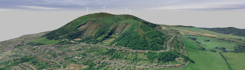
IMPACT: The ability to visualise the proposed scheme in 3D, with or without draped aerial orthophotos, textures and heighted features is an important precursor to many EA studies. It can also be of particular use when presenting a scheme for planning approval much later in the EA cycle. A realtime 3D fly-through can communicate much more information than a traditional contour plan.

INFLUENCE: Often referred to as the 'Visual Envelope' this indicates whether the development is visible from a single or multiple locations. A simple 'Line of Sight' radiating out from the target defined as a single point, or a counter describing how many targets are visible from selected 'receptors' (eye points) outside the development.

INTRUSION: The degree to which a development intrudes upon the field of view. It is often not sufficient to count the number of targets visible from a particular location, but to take into account the effect distance may have on the degree of intrusion into the field of view of the observer. An object close to the observer may have a greater intrusion than one that is hundreds of metres away.

IMPACT: What does the proposed development look like?

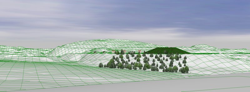
Use LSS 3D view to determine the impact of a development. Utilise heighted point and link features and where an impression of height is required, such as a coppice of trees, use surface codes with a height applied.

Drape digital orthophotos onto the terrain surface for a more realistic view of the terrain. Raster map images may be used in the same way to assist in the orientation of the viewer.

INFLUENCE: Can a single object be seen or not?

Single point line of sight looking outwards from a single pivot point. Specify the height of the pivot point and target above the DTM. Define either a full 360deg sweep or arc between two bearings at a stipulated angular interval. LSS will then draw lines radiating out from the pivot until it reaches the maximum sight distance, the edge of the DTM or a void surface code. As the line goes from visible to invisible along each sight line, LSS will create link features as defined. A correction for earth curvature and refraction is optional. The resulting survey can be over displayed on top of the original survey and/or orthophoto/raster map for a clearer picture of which parts of the DTM are visible and which are invisible from the pivot.

INFLUENCE: How many targets can be seen from a grid of eye points?

Multiple point line of sight looking outwards from any number of points with a common feature code, optionally within a specified surface coded area or all such coded points anywhere in the survey.

This method allows the user to define a grid of 'target' points at a specified grid interval and height above the ground.

The user has full control over the colour banding to define the number of points visible from each grid eye location.

What is produced is a survey containing text boxes whose colour is defined by the number of points visible from the grid point beneath the box and the number contained is the exact counter value. The user may choose a transparent box to enable the display of the DTM behind the ZVI result.

INFLUENCE: Which of the target points are visible from specific locations?

The target counter option (above) has determined that there is line of sight from some receptors to some or all of the target points, but it may be necessary to assess which targets are visible.

The user may select any location within the DTM and LSS will draw lines radiating out towards every visible target point. What is more, because LSS works on a triangular mesh at all times, the user is free to select any point within the DTM and LSS will interpolate the elevation from the triangular mesh.

The user has control over eye and target heights above the DTM and the calculation will take into account any heighted linear or surface obstructions in the way.

INTRUSION: How much of an observer's horizontal field of view is taken up by an object or objects?

It's June 2009 and we have just added another ZVI/ZTV command - 'Horizontal ZTV' which measures how much of a receptor's horizontal field of view is taken up by a development. This is calculated from a user-defined grid of receptors and can measure either the largest contiguous feature visible, the total of all contiguous features or the maximum spread from the furthest left to the furthest right extent of the development. The information is stored as a horizontal angle in degrees. Both this command and 'Visibility Surface' are the only true tests of likely impact because the results reflect the effect that distance has on the apparent size of the object (a large object up-close has more visual impact than the same sized object further away [all things being equal]).

In the above example, we have four distinct objects, A, B, C and D. When viewed from position V at a precision of 2 degrees, object A takes up 9*2deg (18deg), B takes up 7*2deg (14deg) and C & D combine to produce a contiguous area of 14*2 (28deg).

Therefore, the maximum contiguous is 28deg, the total contiguous is 18+14+28=60deg and the total spread is 39*2=78deg. Any of these results can be produced for a user-defined grid of receptors and for a user-defined angular interval.

What is produced is a model where the elevation of every grid point represents the chosen Horizontal ZTV in degrees. It is then possible to contour this or display coloured bands in order to highlight potentially problematic areas of high 'impact'. And remember, in LSS if you add your own heighted links or surfaces into the model, these will act as barriers to the ZTV, thus allowing you to calculate a more realistic picture of the likely impact. And, furthermore, if you are using vector mapping information (such as MasterMap in the UK) LSS is capable of applying surfaces to different features, thus giving you a really quick way to apply heights to objects such as buildings and woodland.

INTRUSION: How much of an observer's vertical field of view is taken up by an object or objects?

Here we define a grid of eye points as above, but we are interested in the degree to which the target(s) fill the viewers field of view as defined

by points within specified surface coded areas. Imagine lines drawn from each eye point, through the DTM to each of the chosen target points. These targets simply define the line to follow from the eye. In fact the sight line itself will continue through each target until it reaches the edge of the surface coded area within which it resides. What will then be calculated at the eye point will be the vertical angle between the lowest and highest point along each sight line (if the target surface is visible along this line). What is actually stored at the eye point is the highest of these values, together with the observation number of the point with the greatest influence. 'Contours' on the resulting LSS model are in fact Isopleths and should prove valuable in the quantification of intrusion across large and small areas alike.

Constraints Mapping

A relatively new option in LSS and it is already proving very popular. Instead of designing a proposed development, how about an analysis which tells you before you start what will be acceptable within the proposed development area? This kind of analysis is called 'Constraints mapping'.

The user defines a grid of points within the area of interest. The grid can be as dense as necessary. Then the user defines as many viewpoints as they wish. LSS will then project an 'horizon' from each viewpoint to each gridpoint in turn.

So, what you are getting is a model within the proposed development area which defines the boundary between what is visible and what isn't from the most critical viewpoint looking into the development. Armed with this model, as long as any development did not protrude through this 'constraints model' then it would not be visible from ANY of the viewpoints.

• Civil Engineering
• Accident and Collision Investigation
• Construction
• Earthmoving
• Golf course construction
• Hydrographic and Dredging
• Land Survey (Geomatics)
• Mine and Quarry
• Waste Management
• Coastal Monitoring
• People and LSS
• Showcasing LSS and its users